Learn How Inertia and coupling stiffness combine to create instabilities in servo axis operation – and what you can do about it.
学习关于 惯量和联轴器刚度的组合 如何 产生伺服轴操作的不稳定,以及如何解决这个问题。
When it comes to motion control, torque alone is not enough. Applications like 300-part-per-minute packaging or web printing require ultrahigh speed operation, accurate positioning, and tight synchronization among dozens of axes.
当谈到运动控制时,仅仅提到扭矩是不够的。例如:300件/min的打包应用 或者 超高速网络打印操作,精确定位,还有多轴间的紧密同步等应用。
Electromechanical systems can provide this degree of performance, but they depend on proper interplay between the mechanical properties and the electrical properties of the system. If an axis has poor mechanical characteristics caused by a high inertia mismatch between load and motor and/or significant compliance (torsional flex) in the coupling, shafts, and belts, mechanical resonances will prevent the electrical controls from performing as required. At best, you might wind up with overshoot and extended settling times; at worst, the axis may fall into runaway oscillation. It doesn’t matter how much torque you have – if your load inertia is too high for your motor and coupling, your system simply will not perform as required.
You may have seen the commercial that shows a pickup truck towing a jumbo jet down a runway. Now imagine that the truck is pulling a free-wheeling jet using an ultra-strong bungee cord. Maybe the truck can generate enough torque to get the plane rolling but it’s pretty obvious that with the combination of inertia mismatch and elastic conditions, there is no way that a vehicle the size of the truck could control that load effectively. Although rules of thumb abound for ratios of load inertia to motor inertia (10:1, 1:1, 5:1, etc.), performance varies from design to design based on systems-level characteristics. Let’s take an analytical look at the issues involved and how they can affect your system.
Servo axes are able to deliver top performance because of the ability of the electrical control and drive system to optimize the mechanical performance based on closed-loop feedback. The controller sends path commands to the servo amplifier (drive), which generates an electrical drive signal that tells the motor when and how to rotate. An encoder or resolver monitors the actual position/speed of the motor, allowing the system to quantify the magnitude and frequency of the error introduced by mechanical issues and external forces. Based on this feedback, the properties of the drive signal can be tuned to optimize the performance of the axis.
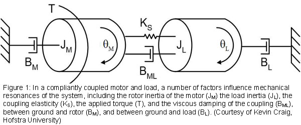
To understand how mechanical issues can affect this process, consider a load connected to a motor via a shaft/coupling (see figure 1). [Note: for purposes of this article, we will confine the discussion to a rotary servo motor with an internal spinning rotor]. We can define the inertia ratio as the driven-load inertia JL and rotor inertia of the motor JM as:
Inertia ratio=JL/JM [1]
In a perfect system with an infinitely stiff motor shaft and coupling, the rotor would spin and turn the load along with it. In reality, all couplings have some degree of compliance. We can model the shaft/coupling as a spring with spring constant Ks. In such a case, when the shaft begins to turn and encounters a high JL, the shaft winds up and the load at best lags the rotor and at worst either moves the opposite direction from the rotor (anti-resonance) or wildly amplifies the force applied by the motor (resonance). The frequencies of these points essentially define the usable bandwidth of the motor across which the system can optimize motion to effectively deliver the load to the commanded position or move it at the commanded velocity.
Let’s take a closer look at how inertia ratio and coupling stiffness interact in our compliantly coupled system to introduce mechanical resonances that degrade motion. We start with the expression for angular acceleration for both the motor and the load.
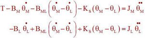
where
JM = rotor inertia of the motor
JL = the load inertia
KS = coupling elasticity
T = applied torque
BML = viscous damping of the coupling
BM = viscous damping between ground and rotor
BL = viscous damping between ground and load
Next, we move the analysis into the frequency domain using the Laplace transform
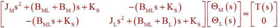
to obtain the equations of motion in terms of the complex frequency s:
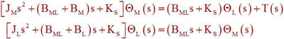
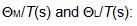
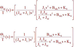
This gives us the transfer functions
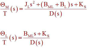
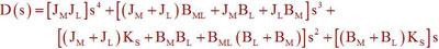
where D(s) represents a denominator function common to both, introduced for simplicity:
We can set BM and BL to zero, since their effect on resonance is negligible. With that change, our transfer functions become:
If we group terms, we obtain:
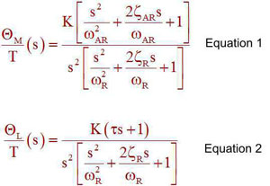
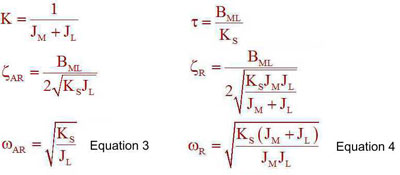
Equation 3 and equation 4 are the key results from this derivation. They are the frequencies of the vibration modes excited in the axis by the interaction between the coupling compliance and the inertias. They are the anti-resonance frequency ωAR and the resonance frequency ωR .
The resonance and anti-resonance peaks of the system identify areas of anomalous behavior. At ωAR , the load moves with an equal and opposite torque from the motor – the two are 180o out of phase. The result is that the motor’s rotor stands still while the load oscillates back and forth. The energy from the motor essentially gets trapped in a subsystem consisting of the load and the compliant coupling. The problem is that most designs attach feedback devices only on the motor, which means that motor might appear broken while the load oscillation may go undetected. At best, load does not complete the commanded motion. At worst, the machine and/or product gets damaged.
At ωR , the motor and load are in phase, so instead of dissipating energy, the system amplifies it. As a result, increasing the gain of the system overall means introducing potentially catastrophic behavior at the resonance peak. This explains why, for example, a beverage line might work perfectly well at 280 parts per minute but when it’s bumped up to 300, it starts flinging bottles across the room.
Now let’s take a closer look at how anti-resonance and resonance spikes can potentially interfere with the tuning process and was system performance. Under normal circumstances, a servo would be tuned by analyzing the feedback and adjusting the drive signal to achieve more or less consistent response across the operating frequencies of interest. This process typically starts with increasing the gain to optimize system response. The problem is that in the curve shown in figure 2, increasing the gain on the drive signal would push the resonance peak up past unity, causing erratic behavior like the bottle flinging.
The standard way to address this issue is to apply a low-pass filter that removes the two spikes (or any secondary resonances, for that matter). This works when the resonances fall at high frequencies, but when they fall at lower frequencies, that filtering technique sacrifices much of the usable bandwidth of the axis. It might be possible to raise the gain but the system might not be able to complete the motion cycle the allotted time. This is the crux of the problem we discussed at the beginning of the article?the motor may have plenty of torque but if the inertia ratio and coupling stiffness are such that resonances crop up at low frequencies, even the best electrical engineer will not be able to make the system operate stably higher speeds. Over time, the industry has mined practical experience and intuitive understanding to develop rules of thumb. That’s not the most effective method of dealing with the problem, however.
“When people talk about rules for inertia mismatch, I say wait a minute, if you have a flexible coupling, you have to understand where the anti-resonance and residences are,” says Kevin Craig, mechatronics specialist and professor of mechanical engineering at Hofstra University (Hempstead, New York). “If you’re trying to control over some frequency range and you stay away from them that’s fine, but if you get close to the anti-resonance or the resonance frequencies, you have to deal with them.”
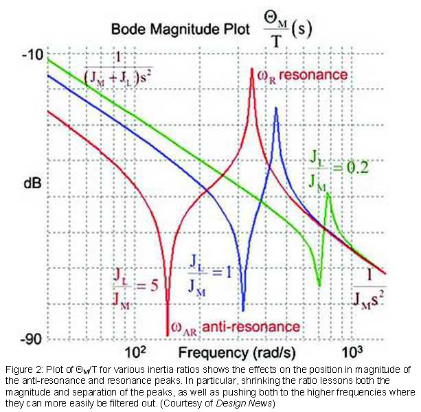
Let’s take a closer look at the Bode plot of ΘM/T(s) (equation 1) to better understand how adjusting inertia ratios can help address the situation. As equations 3 and 4 show, the positions of ωAR and ωR are strongly affected by spring constant and the inertia ratio. The usable bandwidth of the system runs roughly to the shoulder where the plot begins to tip into the anti-resonance peak. Obviously, the higher the upper bound of the bandwidth, the greater the system response.
Take a close look at the three curves. As the inertia ratio drops, both the magnitude and separation of the two resonance peaks drop. More important for our purposes, ωAR and ωR shift to higher frequencies, increasing the bandwidth of the axis. The shift also makes it easier to apply filtering techniques to clean up the signal prior to tuning the loop. At a 1:1 ratio, for example, the peaks move to high enough frequencies that we can remove them with a low pass filter and then apply tuning techniques to flatten out the gain. Alternatively, inertia ratio and coupling stiffness can be used push the two peaks sufficiently close together that it is possible to apply a notch filter to remove one or more peaks prior to tuning the servo.
“I could never understand inertia mismatch because it’s all a matter of knowing what the stiffness is, knowing what the inertia ratio is, then looking at the Bode plots and staying. ‘What am I trying to do? What’s the bandwidth of my controller? How am I trying to control this load?’” says Craig. “I could never put down a rule and say, ‘It’s got to be this.’ I never understood that approach.”
Addressing resonance frequencies
To boost the frequency of the natural resonance, we can increase the spring constant or modify the inertia ratio by either increasing motor size or decreasing load inertia. Working with a more powerful motor typically adds to cost, size, weight, and energy consumption. Using the stiffest possible shaft for the coupling can improve the situation, but here, too, there are drawbacks. Ultra-stiff shafts require very accurate installation. Any alignment errors can cause premature wear on the bearings, leading to early failure.
Another method is to reduce the inertia mismatch by adding mass to the rotor, which is the source of JM. It does not change the torque of the system but it does damp the motor’s response to the coupling. “You’ve slowed down the response of the motor, and since the motor responds slower it is less prone to vibration when you turn your gain up,” says Steve Huard, staff engineer at Parker Hannifin (New Ulm, Minnesota). “That’s another way of fixing the problem.” On the downside, this reduces system response.
Direct-drive motors provide another solution for the right application. Also known as frameless or kit motors, these designs involve making the motor a part of the load. One example would be a conveyor belt for which the rotor of the motor protects out as the axle for the belt. In such a case, KS rises toward infinity. These designs can tackle enormous inertia mismatches and still position effectively. On the downside, they are more complex to install and very unforgiving of misalignment. They may work well in robotic arms, for example, but in a factory environment that relies on maintenance staff handle replacing failed components, they may not be a good fit.
Reduction ratios and reflected inertia
Another way to address the issue of load inertia is to add a gearhead. We define the gear ratio N for two gears as the ratio of their diameters:
N=D_2/D1
If we attach a motor producing torque τ2 at speed ω1 ,our output torque τ2 and angular velocity ω2 are given by:
\tau_2=\tau_1\cdot N\\
\omega_2=\omega_1/N
Meanwhile, the gearhead scales the load inertia “seen” at the motor shaft as:
J_{reflect}=J_L/N^2In other words, the addition of the gear reducer boosts the torque linearly but reduces the reflected inertia affecting resonance by 1/N2. “Reduction ratio is kind of the magic bullet,” says Bryan Knight, automation solutions team leader, Mitsubishi Electric (Vernon Hills, Illinois). “Sometimes going to a smaller motor and better gearing can give you a better inertia mismatch.” A standard 3:1 gearhead could reduce a potentially troublesome 54:1 inertia mismatch to 6:1, for example, while increasing torque by a factor of three at the load side.
You might assume that adding a reduction ratio would also had cost, but that’s not necessarily true. “If you use a gearhead to do inertia matching, you can reduce your cost and overall size compared to using a motor alone,” says Jeff Nazzaro, servo and gearhead manager for Parker Hannifin. “We have shown examples of an application that needed a 142-mm frame size motor. If you add a gearhead, you can drop the overall frame size down to 90 mm and also save a good 35% to 40% in the cost of the whole system. The gearhead is an added cost but the motor gets smaller and you can go with a smaller drive, too.”
That said, the approach has to be considered within a systems context, including load speed and torque multiplication. Gearheads have maximum input speeds, typically 6000 RPM and below. A gearhead might be able to effectively rescale a 10:1 inertia ratio in an application with moderate speed and consistent load but if you use it in a spindle application operating at 60000 RPM, it won’t survive. Applying that same design at a lower speed to correct a 100:1 ratio on an application like a conveyor belt could also create problems. “As you use higher gear ratios to get better and better inertia ratios, you create higher torque multiplication through the gear train,” Nazzaro notes. “If your conveyer belt jams and you’re not current limiting your motor, you will strip the gear train.”
Using gearheads involves other trade-offs. As mechanical components, they may require maintenance like lubrication or replacement of seals. They add length and introduce audible noise. Lifetime depends on load, gearhead type, duty cycle, etc. but they’ll typically need replacing after several years of operation.
There’s another issue that arises related to speed. For systems with high reduction ratios and rapid deceleration, the regenerative energy produced is very high. Although this can be beneficial for energy sharing among multiple axes operating on a common DC bus, for example, it can also be problematic in the case of an emergency stop or line stoppage. “You’re limited by the amount of energy you can dissipate,” says Knight. “You don’t have anything that can absorb the energy because all the axes are stopping at the same time, but all of that energy has to go somewhere.”
A process that undergoes an emergency stop a few times a month or a quarter, for example, might not be a problem but a line programmed to stop when a product is missing or defective might stop multiple times a shift. “You chose a high gear ratio to get away with a smaller motor that still has plenty of torque but your regenerative braking energy, which you have to dissipate with its own braking resistor, goes up tremendously,” he adds. “This is where sizing software becomes important as it helps identify motor and gear reduction combinations that provide the right torque and speed for the application, while minimizing inertia ratio and wasted regenerative energy.”
Designing at the system level
The most straightforward method for arriving at the ideal system is to begin by determining the appropriate size of directly coupled motor to do the job. Frequently, this requires an unacceptably large motor. In that case, determine whether a gearhead can be used to reduce the load inertia so that it will deliver acceptable performance in terms of resonances. This should allow you to rescale the motor/drive. From there, it’s a matter of iterating to find the best combination for your application, keeping in mind issues of speed, torque multiplication, etc. If your system cannot permit the use of a gearhead, then a direct drive motor may be your best choice. This is the general methodology used by most motor sizing programs.
Any time you’re working with a product engineer or a motor sizing program, make sure that you understand the assumptions on which are operating. Those 10:1 or even 5:1 rules of thumb are based on an intuitive understanding based on experience, but may not take into account the fact that the real problem comes from the interaction of the inertias and the coupling. Particularly in systems pushing the performance envelope, rules of thumb are not likely to be successful. “I don’t think anything replaces a good model and understanding of your system and application,” says Craig. “What you’re doing with these rules of thumb is saying that you’re not willing to understand what’s really happening.”
Motion control is a systems-level function and should be evaluated from a systems perspective. Don’t just boost your motor size by 10% or 20% over that of the previous platform, take the time to understand the effects of inertia ratio, compliance, speed, etc. before settling on your design. Develop a system that takes into account the factors we’ve discussed above, and make sure that you understand how it will function. The best way to do this is for the mechanical design team to work with the electrical and controls engineers to establish components and parameters that will best serve the application. Using an integrated, system-level approach in the beginning will help prevent frustration and unexpected problems later on.
FURTHER READING
K. Craig, “Inertia Mismatch: Fact or Fiction?” Design News, 2/2013.
G. Ellis, “Cures for Mechanical Resonance in Industrial Servo Systems,” IEEE Industry Applications Conference, 9/2001.
G. Ellis, “How to Work with Mechanical Resonance in Motion Control Systems,” Control Engineering, 4/2000.
ACKNOWLEDGMENTS
Thanks go to Kevin Craig for the detailed derivation.
参考文献: